Following up on the post on binomial trees, here’s an overview of binomial heaps and the mechanisms behind their various operations.
Structure
A binomial heap is merely a collection of binomial trees, each of which satisfy the heap invariant, having either 0 or 1 tree for each order  . A typical way to represent this is collection is a linked list where the
  th node has as its value either null or a binomial tree of order .
Recall that a binomial tree of order has exactly  nodes and depth . This results in a direct analogy between the representation of a number
  in binary and the structure of the binomial heap with nodes. For instance, the number 13 has the unique binary representation 1101. This means that the binomial heap with 13 nodes is uniquely determined to have 1 binomial tree each of orders 0, 2, and 3. (
 .) An example of such a heap is shown below (minus the linked list pointers):
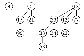
Source: https://en.wikipedia.org/wiki/Binomial_heap
Note that this also implies that a heap with nodes with be represented by  trees.
Operations
Merge
The  operation of merging two binomial heaps is not only their main advantage over traditional binary heaps, but is essential to how most other operations are accomplished.
The crucial aspect of how the merge operation works is that merging two binomial trees of order , each being heaps, takes  time. You can simply add the one with a larger root value as a child of the other to get a valid tree-heap of order
  . This is illustrated below with two trees of order 2:

Source: https://en.wikipedia.org/wiki/Binomial_heap
Because of this, one can merge 2 binomial heaps with elements in  time, following essentially the same procedure as adding 2 binary numbers (keeping track of a ‘carry’ tree, analogous to a carry digit). The figure below illustrates the merging of two binomial heaps with 11 and 3 elements, respectively.
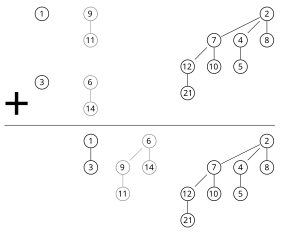
Source: https://en.wikipedia.org/wiki/Binomial_heap
The analogous binary addition would be adding the numbers 1011 and 0011 to get 1110.
Insert
Insertion of a new element into a heap can be simply accomplished by creating a new heap with just the one tree/element and merging it with the original. This takes time for a single operation, but amortized time when taken over the course of consecutive insertions. (Think of the time to increment a binary number by 1 times.)
Find Min (Peek)
Since there are at most  trees in a heap with nodes, finding the min by just iterating over the trees takes time. This is the main disadvantage to a binary heap.
Remove Min (Pop)
However, removing the minimum element takes time, just as with a binary heap. Having found the tree with the min as its root, you can split up its children into a separate binomial heap and simply merge this with the original.
Set Priority
Setting/modifying the value of an element takes time, since you just float it up or sink it down its tree as you would with an ordinary heap, and each tree has depth . However, this assumes you have a pointer to where the element is stored.
Delete Element
To delete an element (again assuming you know where it is), you can simply set its priority to  and remove the min from the heap.
 , where
  is the number of bits flipped in increment
  . We have:

 on a non-empty sequence
  returns a copy of


 norm and
  ‘norm’ of a binary vector.
 is simply
  .
. time, where
  , where
  is the complexity of any multiplication algorithm used, precisely by reducing division to multiplication.
 and
and  , finds the quotient
  such that
  by:
by: of
of  (by performing the multiplicative iteration
  )).
)). by
by  : the number of bits in the number. Using this upper bound, though, the maximum runtime of incrementing 0
 .
. can be defined recursively as follows:
 is a tree with a single root node and no children.
 .
.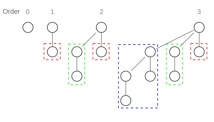
 and assigning one as the leftmost child of the other. This is apparently the property which makes them useful for merging two of them in the context of binomial heaps, but I’ll have to get to that in a later post.
 nodes at depth
  .
. and
and  , respectively.